3. Gates

This course is derived from the course Biological Circuit Design by Michael Elowitz and Justin Bois, 2020 at Caltech. The original course material has been changed by Matthias Fuegger and Thomas Nowak.


Let's load some libraries we will need.

Feed forward loop (FFL)

A motive commonly found in cells like E. coli is the so called feed forward loop (FFL). The name is unfortunately misleading since it has convergent paths, but not a loop - we will nonetheless use it since it is established in literature.

The motive comprises of 3 species, let's call them $X,Y,Z$, and three interactions among them along two paths:

\begin{align} &X \rightarrow Y \rightarrow Z\\ &X \quad \rightarrow \quad Z \end{align}

We think of $X$ as a circuit input and $Z$ as its output. Interactions can be activating and repressing, which we will denote by $X \to Y$ for an activating interaction and $X -\mid Y$ for a repressing interaction of $X$ on $Y$.

We say a path is activating if the number of repressing interacting along it is even. It is repressing otherwise.

Following literature, we call a FFl coherent if both paths are either activating or repressing and incoherent if one is repressing and the other activating.

FFL types

There are a total of $2^3 = 8$ different FFLs depending on which of the interactions are activating and repressing. All are shown below, in a figure taken from Alon, Nature Rev. Genet., 2007.

FFL classes

The figure also indicates common abbreviations for these circuits: e.g., C2-FFL is the coherent FFL of type 2 and I4-FFL is the incoherent FFL of type 4.

The most-encountered FFLs

While FFLs in general are motifs, some FFLS are more often encountered than others. In the figure below, also taken from the Alon review, we see relative abundance of the eight different FFLs in E. coli and S. cerevisiae. Two FFLs, C1-FFL and I1-FFL stand out as having much higher abundance than the other six.

![FFL abundance](figs/i1-ffl.png)

We will take a look at these two FFLs in turn to see what features they might provide. First, though, we need to consider the logic of regulation by more than one transcription factor.

Logic of regulation by two transcription factors

Because X and Y both regulate Z in an FFL, we need to specify how they do that. For the sake of illustration, let us assume we are discussing C1-FFL, where

$$ Y \rightarrow Z\\ X \rightarrow Z $$

We distinguish between two semantics:

So, to fully specify an FFL, we need to also specify the logic of how Z is regulated. So, we might have, for example, a C1-FFL with OR logic. This gives a total of $2 \cdot 8 = 16$ possible FFLs.

We are now left with the task of mathematically modeling AND and OR logic.

Logic with two activators

Assume that $z = f_{AND}(x,y)$ is the normalized (within $[0,1]$) steady state input-output behavior of Z = X AND Y. Likewise, $z = f_{OR}(x,y)$ is the normalized steady state input-output behavior of Z = X OR Y.

Let $f$ be either $f_{AND}$ or $f_{OR}$. The dynamics of the concentration of $Z$ may then be written as

\begin{align} \frac{\mathrm{d}z}{\mathrm{d}t} = \beta_0\,f(x, y) - \gamma z\enspace, \end{align}

where $\beta_0$ is the maximal production rate and $\gamma$ is its degradation/dilution rate.

Our goal is to specify the dimensionless function $f(x, y)$ that encodes the appropriate logical functions. There are two ways we can come up with a candidate function:

Remember from Lecture 1 (chapter Activation) that for an activator $X$, the approximate production rate of the regulated $Z = f(X)$ was \begin{align} \beta(X) = \beta_0 \frac{X/K_\mathrm{d}}{1+X/K_\mathrm{d}} \enspace, \end{align} where $\beta_0$ is the maximal production rate and $K_d$ the dissociation constant $k_-/k_+$. Generalizing this to higher order Hill coefficients $n \geq 1$ we can write \begin{align} \beta(X) = \beta_0 \frac{(X/K_\mathrm{d})^n}{1+(X/K_\mathrm{d})^n} \enspace, \end{align} The result is a sharper, say "more digital", dependency of the production rate with respect to the activator $X$.

A natural generalization to two inputs is to form the AND by multiplying and the OR by adding $(X/K_\mathrm{d})^n$ terms as follows:

\begin{align} f_{AND}(x,y) &= \frac{(x/k_x)^{n_x} (y/k_y)^{n_y}}{1 + (x/k_x)^{n_x} (y/k_y)^{n_y}}\\[1em] f_{OR}(x,y) &= \frac{(x/k_x)^{n_x} + (y/k_y)^{n_y}}{1 + (x/k_x)^{n_x} + (y/k_y)^{n_y}} \enspace. \end{align}

In what follows, we will substitute $x/k_x \to x$ and $y/k_y \to y$ such that $x$ and $y$ are now dimensionless, nondimensionalized by their Hill $k$. In this notation, we have

\begin{align} f_{AND}(x,y) &= \frac{x^{n_x} y^{n_y}}{1 + x^{n_x} y^{n_y}}\\[1em] f_{OR}(x,y) &= \frac{x^{n_x} + y^{n_y}}{1 + x^{n_x} + y^{n_y}} \enspace. \end{align}

We can make plots of these functions to demonstrate how they represent the respective logic.

Here, purple indicates that $f(x, y) = 0$ (low) and yellow indicates that $f(x, y) = 1$ (high).

Logic with two repressors

Now let's consider the case where we have two repressors, as in the C3-FFL or I2-FFL. The AND case where X and Y are both repressors is (NOT X) AND (NOT Y) = NOR(X,Y). Here, either repressor (or both) can shut down gene expression. Logic gates that work in this way are used in synthetic designs for their ease of design and possibilities to vary input and output species. We come to this later.

For the OR of two repressors, we have (NOT X) OR (NOT Y) = NAND(X,Y). We might get this kind of logic if the two repressors need to work in concert, perhaps through binding interactions, to affect repression.

We can encode these two input-output functions with dimensionless Hill regulation functions

\begin{align} f_{NOR}(x,y) &= \frac{1}{(1 + x^{n_x}) (1 + y^{n_y})}\\[1em] f_{NAND}(x,y) &= \frac{1 + x^{n_x} + y^{n_y}}{(1 + x^{n_x}) ( 1 + y^{n_y})}\enspace. \end{align}

The NOR gate

Since the NOR gate is of great practical relevance we will also provide a derivation for its steady state input-output approximation.

Assume that two repressors $X$ and $Y$ bind respective binding sites $P_X$ and $P_Y$ of a promoter $P$. Only if neither is present, a protein will be produced. We have, \begin{align} f_{NOR}(x,y) = \frac{P}{P^{tot}}\enspace, \end{align} where $P^{tot} = P + P^{occ}$ is the total number of promoters with $P^{occ}$ being the number of promoters occupied by either $X$ or $Y$. In particular, since $X$ and $Y$ are independent, the fraction of promoters that are free is the product of the fractions of promoters that have free $X$-binding-sites and those that have free $Y$-binding-sites. Thus, with \begin{align} K^d_x &= \frac{P_x \cdot x}{K^{occ}_x}\\ K^d_y &= \frac{P_y \cdot y}{K^{occ}_y}\enspace. \end{align} it is \begin{align} \frac{P}{P^{tot}} = \frac{1}{1+\frac{x}{K^d_x}} \cdot \frac{1}{1+\frac{y}{K^d_y}} = f_{NOR}(x,y)\enspace, \end{align} with Hill coefficients $1$.

Let's make some plots to see how these functions look.

Logic with one activator and one repressor

Now say we have one activator (which we will designate to be A) and one repressor (which we will designate to be R). Now, AND logic means A AND (NOT R), and OR logic means A OR (NOT R).

The dimensionless regulatory functions are

\begin{align} f_{ANDNOT}(x,y) &= \frac{x^{n_x}}{1 + x^{n_x} + y^{n_y}}\\[1em] f_{ORNOT}(x,y) &= \frac{1 + x^{n_x}}{1 + x^{n_x} + y^{n_y}}\enspace. \end{align}

Finally, let's look at a plot.

A word of warning

The above generalized Hill functions for two inputs have been deemed useful in phenomenologically describing gates. They should not be interpreted as the way to model AND/OR combinations of activators/repressors. Your concrete genetic circuit may require a different function to describe normalized steady-state input-output behavior.

Dynamical equations for FFLs

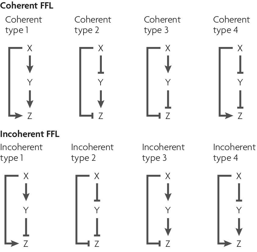
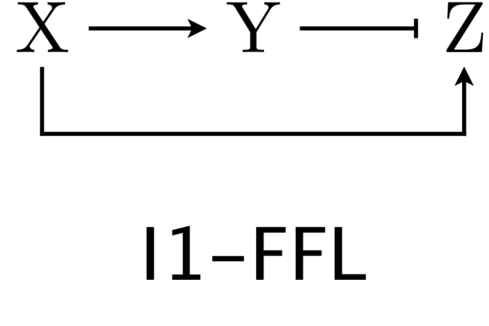
To analyze the C1-FFL and I1-FFL (or any of the other FFLs), in response to changes in the input X, we can write a generic system of ODEs for the concentrations of Y and Z. We know that Y is either activated or repressed by X and itself experiences degradation. We define a dimensionless function $f_y(x/k_{xy}; n_{xy})$ to describe the activating or repressive Hill function for the regulation of X by Y. We have used the notation that $n_{ij}$ is the Hill coefficient for j regulated by i, with $k_{ij}$ similarly defined. To be explicit:

The dynamical equation for $y$ for either activating or repressive action by X is

\begin{align} \frac{\mathrm{d}y}{\mathrm{d}t} &= \beta_y\,f_y(x/k_{xy}; n_{xy}) - \gamma_y y. \end{align}

Similarly, we define the dimensionless function $f_z(x/k_{xz}, y/k_{yz}; n_{xz}, n_{yz})$ to describe the regulation in expression of Z by X and Y. This have any of the functional forms we have listed above for activation/repression pairs and AND/OR logic. The dynamical equation for $z$ is then

\begin{align} \frac{\mathrm{d}z}{\mathrm{d}t} &= \beta_z\,f_z(x/k_{xz}, y/k_{yz}; n_{xz}, n_{yz}) - \gamma_z z. \end{align}

We can nondimensionalize these equations by choosing

\begin{align} t &= \tilde{t} / \gamma_y, \\[1em] x &= k_{xz}\,\tilde{x},\\[1em] y &= k_{yz}\,\tilde{y},\\[1em] z &=z_0\,\tilde{z}, \end{align}

where $z_0$ is as of yet unspecified. Inserting these expressions into the dynamical equations gives

\begin{align} \gamma_y k_{yz}\,\frac{\mathrm{d}\tilde{y}}{\mathrm{d}\tilde{t}} &= \beta_y\,f_y\left(\frac{k_{xz}}{k_{xy}}\,\tilde{x}; n_{xy}\right) - \gamma_y k_{yz} \tilde{y},\\[1em] \gamma_y z_0\,\frac{\mathrm{d}\tilde{z}}{\mathrm{d}\tilde{t}} &= \beta_z\,f_z(\tilde{x}, \tilde{y}; n_{xz}, n_{yz}) - \gamma_z z_0 \tilde{z}. \end{align}

If we conveniently define $z_0 = \beta_z/\gamma_z$, then the dynamical equations become

\begin{align} \frac{\mathrm{d}\tilde{y}}{\mathrm{d}\tilde{t}} &= \beta\,f_y\left(\kappa\tilde{x}; n_{xy}\right) - \tilde{y},\\[1em] \gamma^{-1}\,\frac{\mathrm{d}\tilde{z}}{\mathrm{d}\tilde{t}} &= f_z(\tilde{x}, \tilde{y}; n_{xz}, n_{yz}) - \tilde{z}, \end{align}

where we have defined

\begin{align} &\beta = \frac{\beta_y}{\gamma_y k_{yz}},\\[1em] &\gamma = \frac{\gamma_z}{\gamma_y}, \\[1em] &\kappa = \frac{k_{xz}}{k_{xy}}. \end{align}

In addition to the Hill coefficients, these dimensionless parameters complete the parameter set of the FFL dynamical system. Each has a physical meaning. The parameter $\beta$ is the dimensionless unregulated steady state level of $y$, $\gamma$ is the ratio of the decay rates of Z and Y, and $\kappa$ is the ratio of the amounts of X that are necessary to regulate Z and Y.

Henceforth, we will work with these dimensionless equation and will drop the tildes for notational convenience.

Numerical solution of the FFL circuits

To specify the dynamical equations so that we may numerically solve them, we need to specify the functions $f_y$ and $f_z$ along with their Hill coefficients. The function $f_y$ is either an activating or repressive Hill function, and the functions $f_z$ have already been defined as aa_and(), aa_or(), etc., above. For convenience in future lessons, these functions are included in the biocircuits.reg submodule.

Let's proceed to code up the right-hand side of the dynamical equations for FFLs. It is convenient to define a function that will give back a function that we can use as the right-hand side we need to specify to scipy.integrate.odeint(). Remember that odeint() requires a function of the form func(yz, t, *args), where yz is an array of length containing the values of $y$ and $z$. For convenience, our function will return a function with call signature rhs(yz, t, x), where x is the value of $x$ at a given time point.

To study the dynamics, we will investigate how the circuit responds to a step up in concentration of X, assuming all concentrations are initially zero, and how a circuit at steady state with nonzero concentration of X responds to a step down in X to zero. This case is particularly relevant for a C1-FFL and an I1-FFL, since in the absence of X (and leakage), the steady state levels of both Y and Z are zero. For other FFLs, the steady state concentrations of Y or Z absent X can be nonzero. In this case, you can think of the sudden rise in X being associated also with a sudden rise of effectors that allow Y and Z to turn on.

Now we can write a function to solve the ODEs. Because the steps are discontinuous, we need to solve the ODEs in a piecewise manner. We specify that the step up starts at $t = 0$, and we will allow the time of the step down to be specified. The magnitude of the step up, $x_0$ will also be specified.

Finally, we can write a function to solve and plot the dynamics of an FFL for a unit step.
At the end of this notebook, we have a dashboard to explore the C1-FFL and I1-FFL, but for the pedagogical purposes of exposing design principles here, we will vary the parameters one-by-one as we work down the notebook.

The C1-FFL circuit enables sign-sensitive delay

Now that we have laid the computational groundwork, we will proceed to an analysis of the first of the two over-represented FFLs, the C1-FFL. For reference, the dimensionless dynamical equations are

\begin{align} \frac{\mathrm{d}y}{\mathrm{d}t} &= \beta\,\frac{(\kappa x)^{n_{xy}}}{1 + (\kappa x)^{n_{xy}}} - y, \\[1em] \gamma^{-1}\frac{\mathrm{d}z}{\mathrm{d}t} &= \frac{x^{n_{xz}} y^{n_{yz}}}{1 + x^{n_{xz}} y^{n_{yz}}} - z. \end{align}

Now, let's look at the dynamics for a sudden step up and step down in X.

With these convenient functions available, we can now specify parameters, solve, and plot.

Notice that there is a time delay for production of $Z$ upon stimulation with $X$. This is a result of the AND logic. Though $X$ has immediately come up, we have to wait for the signal to pass through $Y$ for $Z$ to come up. This off-response is perhaps more apparent if we normalize the signals.

Here, the delay is more apparent, as is the fact that both Y and Z have their levels immediately decrease when the X stimulus is removed. So, we have arrived at a design principle: The C1-FFL with AND logic has an on-delay, but no off-delay.

The magnitude of the delay can be tuned

How might we get a longer delay? If we decrease $\kappa = k_{xz}/k_{yz}$, we are increasing the disparity between the threshold levels needed to turn on gene expression. This should result in a longer time delay. Let's try it!

Making a sweep

Indeed, the delay is longer with small $\kappa$. We can quantify how the delay changes with $\kappa$ by plotting how long it takes for the $z$ level to rise to five percent of its steady state value for various values of $\kappa$.

The delay does not change substantially, only about a factor of three over many orders of magnitude.

The C1-FFL with AND logic and filter out short pulses

Now, let's see what happens if we have a shorter pulse. Due to its similarly with the cascade we previously studied, the delay feature of the C1-FFl should also filter our short pulses.

The shorter pulse is ignored in the Z-response because of the delay.

The sign-sensitivity of the delay is reversed with OR logic

We will now investigate the response of the circuit to the same stimulus, except with OR logic.

Again, let's normalize to see it more clearly:

Sign sensitive delay is observed experimentally

The arabinose and lac systems in E. coli are both turned on by cyclic AMP (cAMP), which stimulates production of CRP, but they have different architectures, shown below.

araBAD and lacZYA

In both system where multiple species regulate one, AND logic is employed.

Mangan an coworkers (J. Molec. Biol., 2003) performed an experiment where they put a fluorescent reporter under control of the products of these two systems, araBAD and lacZYA, respectively. In the lac system, IPTG was also present, so LacI was inhibited. Thus, lacZYA production was directly activated by CRP. Conversely, the arabinose system is a C1-FFL.

They measured the fluorescent intensity in cells that were suddenly exposed to cAMP. The response of these two systems to the sudden jump in cAMP is shown in the left plot below.

response to steps

While the lac system response immediately, the arabinose system exhibits a lag before responding. This is indicative of a time delay for a step on in the stimulus for a C1-FFL. Conversely, after these systems come to steady state and are subjected to a sudden decrease in cAMP, both the arabinose and lac systems respond immediately, without delay, which is also expected from a C1-FFL with AND logic.

Kalir and coworkers (Mol. Sys. Biol., 2005) did a similar experiment with another C1-FFL circuit found in E. coli, this time with OR logic. A circuit that regulates flagella formation is a "decorated" C1-FFL, shown below. We say it is decorated because the "Y" gene, in this case FliA, is also autoregulated. Importantly, the regulation of FliL by FliA and FlhDC is governed by OR logic.

fliA system

Kalir and coworkers used engineered cells in which the FlhDC gene was under control of a promoter which could be induced with L-arabinose, a chemical inducer. The gene product FliL was altered to be fused to GFP to enable fluorescent monitoring of expression levels. To consider a circuit where FlhDC directly activates FliL, Kalir and coworkers used mutant E. coli cells in which the fliA gene was deleted.

Because of the OR logic, we would expect that a sudden increase in FlhDC would result in both the wild type and mutant cells to respond at the same time, that is with no delay. Fluorescence traces from these experiments are shown in the left plot, below.

response to steps fliA

Both strains show a delay, which is due to waiting for FlhDC to be activated, but both come on at the same time. Conversely, after the inducer is removed and FlhDC levels go down, the system with the wild type C1-FFL circuit shows a delay before the FliL levels drop off, while the mutant does not. This demonstrates the sign-sensitivity with OR logic.

The I1-FFL with AND logic is a pulse generator

We now turn our attention to the other over-represented circuit, the I1-FFL. As a reminder, here is the structure of the circuit.

FFL abundance

X activates Y and Z, but Y represses Z. We can use the expressions for production rate under AND and OR logic for one activator/one repressor that we showed above in writing down our dynamical equations. Here, we will consider AND logic. The dimensionless dynamical equations are

\begin{align} \frac{\mathrm{d}y}{\mathrm{d}t} &= \beta\,\frac{(\kappa x)^{n_{xy}}}{1+(\kappa x)^{n_{xy}}} - y,\\[1em] \gamma^{-1}\,\frac{\mathrm{d}z}{\mathrm{d}t} &= \frac{x^{n_{xz}}}{(1 + x^{n_{xz}} + y^{n_{yz}})} - z. \end{align}

For this circuit, we will investigate the response in Z to a sudden, sustained step in stimulus X. We will choose $\gamma = 10$, which means that the dynamics of Z are faster than Y.

We see that Z pulses up and then falls down to its steady state value. This is because the presence X leads to production of Z due to its activation. X also leads to the increase in Y, and once enough Y is present, it can start to repress Z. This brings the Z level back down toward a new steady state where the production rate of Z is a balance between activation by X and repression by Y. Thus, the I1-FFL with AND logic is a pulse generator.